The Implications of Energy Loss

To illustrate the shortcomings of the Runge-Kutta method, let’s analyze the Newtonian equations of motion for a planet in orbit around a star:

Here, the star (specifically, the system's center of mass) is positioned at the origin, with ( G ) representing the gravitational constant and ( M ) denoting the star's mass. To utilize Runge-Kutta effectively, we must transform the second derivatives into first derivatives:

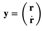
This transformation leads us to the canonical equation form, suitable for common differential equation solvers:

Next, we will implement the fourth-order Runge-Kutta method using Python. For this simulation, we assume that at ( t=0 ), the planet is located on the x-axis, one astronomical unit from the origin, and possesses an initial velocity intended to maintain a circular orbit. We will project the motion for five years into the future.

The resulting trajectory appears as follows:

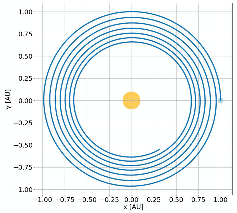
As evident, the planet spirals toward the star, indicating a significant loss of energy. This behavior is problematic, as orbits should conform to closed elliptical paths, as defined by Kepler's laws. The energy in this scenario can be expressed as:

In Python, we can represent the energy calculation as follows:

m = 5.972E24 # kg, mass of Earth

def energy(xyz, vel):

r = np.sqrt(xyz[0]**2 + xyz[1]**2 + xyz[2]**2)

return m/2 * (vel[0]**2 + vel[1]**2 + vel[2]**2) - G*m*M/r

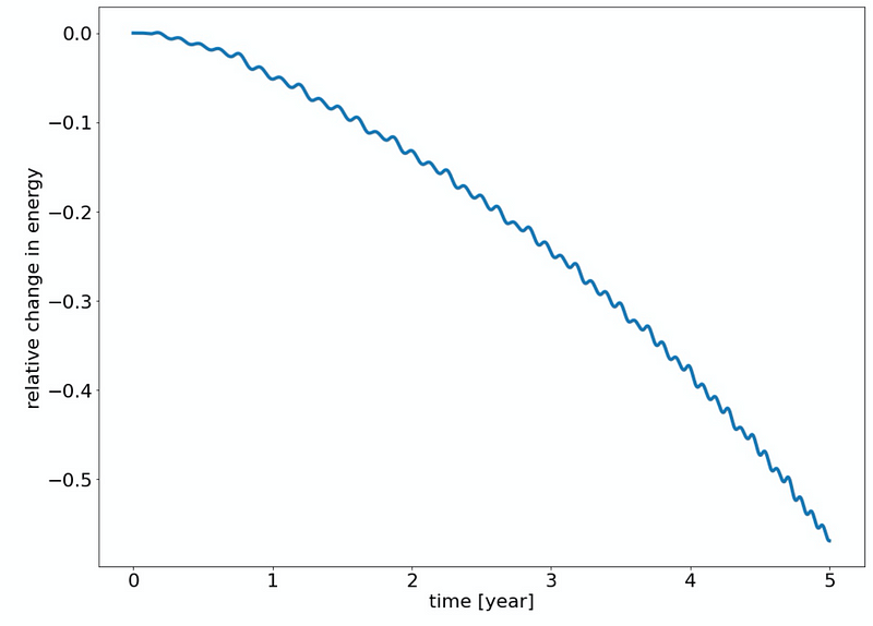
Clearly, we observe a drift in energy, which contradicts the principle of conservation in a static potential. While this issue may not seem critical for short-term simulations, it can lead to significant errors over extended periods.

Addressing the Energy Conservation Issue

An immediate solution might be to opt for a higher-order method, easily achieved by changing the method selection key in SciPy. However, this merely postpones the same issue, as even more advanced Runge-Kutta solvers will eventually exhibit the same energy loss. Alternatively, there exists a category of solvers known as symplectic solvers, which inherently conserve energy—or more accurately, they maintain the volume in phase space. One of the simplest symplectic methods is the leapfrog algorithm, which can be expressed as follows:

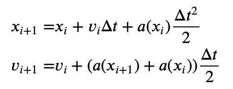
The leapfrog algorithm operates in a two-step iteration: first, it computes new positions using the previous velocity and acceleration. Next, it updates the acceleration based solely on the new position before calculating the new velocities as an average of the old velocity and the newly computed acceleration. Though this method is only second-order accurate, it remains a popular choice, especially in molecular dynamics.

In the context of planetary motion, the implementation yields the following results:

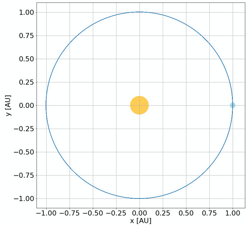
This outcome appears significantly more plausible. Analyzing the energy over the same five-year span reveals:

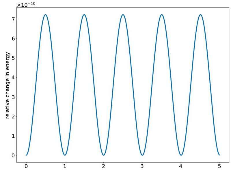
Notably, the y-axis scale indicates that the relative change in energy is on the order of one in ten billion, showcasing remarkable stability. Typically, with symplectic solvers, energy oscillates around the true value instead of drifting away—this characteristic is especially advantageous for long-term simulations.