Section 1.1: Grayscale Conversion

To start, we will import the necessary libraries:

import os

import cv2

import matplotlib.pyplot as plt

Next, we will locate the image on our computer and load it into our program:

path = r’C:UserDocumentsgerdoo’

os.chdir(path)

file = path + ‘image.jpg’

image = cv2.imread(file, cv2.IMREAD_UNCHANGED)

gray = cv2.cvtColor(image, cv2.COLOR_BGR2GRAY)

The final line converts the original image into grayscale. Note that the OpenCV function uses the BGR format rather than the more common RGB format. Now, let’s display the original and the grayscale images side by side:

fig, ax = plt.subplots(1, 2, figsize=(10, 5))

ax[0].imshow(cv2.cvtColor(image, cv2.COLOR_BGR2RGB))

ax[0].axis("off")

ax[1].imshow(cv2.cvtColor(gray, cv2.COLOR_BGR2RGB))

ax[1].axis("off")

plt.show()

The output should resemble the following:

FIG. 2 — The original image converted to grayscale.

Section 1.2: Noise Reduction

Next, we aim to minimize noise in the grayscale image, enhancing the quality of our results. This can be achieved by applying a Gaussian blur, which acts as a smoothing filter. Here’s how to do it:

blur = cv2.GaussianBlur(gray, (3, 3), cv2.BORDER_DEFAULT)

This single line of code demonstrates the power of libraries like OpenCV and SciPy that simplify complex processes.

FIG. 3 — The grayscale image after applying Gaussian blur.

You may not observe significant changes in this simple image.

Section 1.3: Gradient Calculation

The gradient calculation is crucial for most edge detection methods. It represents the directional change in image intensity. For those familiar with physics, think of the gradient as a way to measure the steepest incline of a scalar field.

We can employ Sobel or Scharr methods for this calculation using OpenCV. Here, I'll use the Sobel method:

grad_X = cv2.Sobel(gray, ddepth=cv2.CV_32F, dx=1, dy=0, ksize=-1)

grad_Y = cv2.Sobel(gray, ddepth=cv2.CV_32F, dx=0, dy=1, ksize=-1)

Note that grad_X computes the gradient in the horizontal direction, while grad_Y computes it in the vertical direction. We then convert these gradients to 8-bit integers:

grad_X = cv2.convertScaleAbs(grad_X)

grad_Y = cv2.convertScaleAbs(grad_Y)

To obtain a combined gradient, we can use the following code:

combined = cv2.addWeighted(grad_X, 0.5, grad_Y, 0.5, 0)

After experimenting with different kernel sizes, I settled on a (3, 3) blur kernel.

FIG. 4 — Combined gradient image showcasing different blur kernel sizes.

Section 1.4: Thresholding

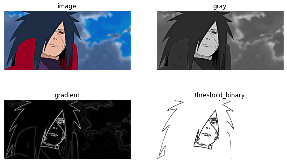
At this stage, we can already observe the prominent edges of the original image, outlining the physical objects and excluding unnecessary details. We can implement thresholding to enhance these strong edges:

ret, threshold_binary = cv2.threshold(combined, 100, 255, cv2.THRESH_BINARY_INV)

Although this appears straightforward, thresholding is a complex topic on its own. The binary thresholding technique yields visually appealing results:

FIG. 5 — The final result of the edge detection process, exactly as envisioned.

Don’t forget, you can create the above subplot using Matplotlib:

fig, ax = plt.subplots(2, 2, figsize=(10, 6))

ax[0, 0].imshow(cv2.cvtColor(image, cv2.COLOR_BGR2RGB))

ax[0, 0].axis("off")

ax[0, 0].title.set_text("Image")

ax[0, 1].imshow(cv2.cvtColor(gray, cv2.COLOR_BGR2RGB))

ax[0, 1].axis("off")

ax[0, 1].title.set_text("Gray")

ax[1, 0].imshow(cv2.cvtColor(combined, cv2.COLOR_BGR2RGB))

ax[1, 0].axis("off")

ax[1, 0].title.set_text("Gradient")

ax[1, 1].imshow(cv2.cvtColor(threshold_binary, cv2.COLOR_BGR2RGB))

ax[1, 1].axis("off")

ax[1, 1].title.set_text("Threshold Binary")

This thresholding exercise was relatively straightforward. More intricate images may require advanced algorithms to tackle their complexity. I hope to delve into those topics in future writings.

Thank you for reading! If you found this helpful, feel free to show your support by clapping, sharing, commenting, or reaching out to me.